Tutorial 2: Quantum Transport in 2D materials#
Introduction#
DPNEGF is a Python package that integrates the Deep Learning Tight-Binding (DeePTB) approach with the Non-Equilibrium Green’s Function (NEGF) method, establishing an efficient quantum transport simulation framework DeePTB-NEGF with first-principles accuracy.
Based on the accurate electronic structure prediction in large-scale and complex systems, DPNEGF implements the high-efficiency algorithm for high-throughput and large-scale quantum transport simulations in nanoelectronics.
Learning Objectives#
In this tutorial, you will learn:
how to extract model for specific systems from baseline model
what is principal layer and how to compute electrode self-energies with DeePTB model
how to compute the transmission spectrum of 2D materials with periodicity in the transverse direction
As demonstrations, we will explore graphene, hBN, and MoS2.
Requirements#
DeePTB and DPNEGF installed. Detailed installation instructions can be found in README.
1. Quantum Transport in Graphene#
Two-dimensional (2D) materials have attracted significant attention in condensed matter physics and nanoelectronics owing to their unique properties.
Graphene is the natural starting point for studying quantum transport in 2D materials. As the first experimentally realized 2D material, it combines a simple lattice structure with unique electronic features such as linear Dirac dispersion and high carrier mobility.
In this section, we will use graphene to introduce the basic steps of quantum transport calculations, including the evaluation of electrode self-energies and transmission spectra. The same methodology will later be extended to hBN and MoS2.
import os
from pathlib import Path
workdir='../../examples/graphene'
wd = Path(workdir)
if not wd.is_dir():
    raise FileNotFoundError(f"Workdir '{wd}' not found. Please adjust 'workdir'.")
os.chdir(wd)
print("\t".join(sorted(os.listdir("."))))
band.json extra_baseline negf.json negf_output_k100 stru_negf.xyz struct.xyz train
from dpnegf.utils.loggers import set_log_handles
import logging
from pathlib import Path


results_path = 'band_plot_api'
log_path = os.path.join(results_path, 'log')
log_level = logging.INFO
set_log_handles(log_level, Path(log_path) if log_path else None)
---------------------------------------------------------------------------
ModuleNotFoundError                       Traceback (most recent call last)
Cell In[2], line 1
----> 1 from dpnegf.utils.loggers import set_log_handles
      2 import logging
      3 from pathlib import Path

ModuleNotFoundError: No module named 'dpnegf'
1.1 Extract system-specific model#
Here we briefly outline the procedure for extracting a system-specific model from the baseline model. For more details, please refer to the DeePTB tutorial.
First, decide on the elements and basis set for the target system. For graphene, we choose the ‘spd*’ for carbon, specified in extra_baseline/c_spd.json. The command dptb esk c_spd.json -o grap_spd_model generates the extracted model sktb.json.
To achieve higher accuracy, we further train the extracted model using sktb.json as the initialization.
The training input file input_templete.json can be automatically generated by: dptb config -m grap_spd_model/sktb.json -tr -sk ./.
After switching to the train directory and copying the input file here as input.json ,the training process can be started with:
dptb train input.json -i ../extra_baseline/grap_spd_model/sktb.json -o train_out.
We recommend that users carefully examine the input.json file to understand the meaning of each parameter.
For 2D materials, the onsite mode should be set to strain, which removes the degeneracy of onsite energies for orbitals with the same angular momentum. It is an essential adjustment for 2D systems. For example, the onsite energies for \(p_x,p_y,p_z\) in graphene should not be identical considering the geometry.
SUMMARY:
In ./extra_baseline:
dptb esk c_spd.json -o grap_spd_modeldptb config -m grap_spd_model/sktb.json -tr -sk ./
In ./train:
dptb train input.json -i ../extra_baseline/grap_spd_model/sktb.json -o train_out
Once training has converged, the resulting model can be loaded to plot and analyze the band structure.
from dptb.nn.build import build_model

model =  "./train/train_out/checkpoint/nnsk.best.pth" # the model for demonstration

model = build_model(model)
DPNEGF INFO    The ['overlap_param'] are frozen!
DPNEGF INFO    The ['overlap_param'] are frozen!
# read the structure
from ase.io import read
structure =  "./train/data/POSCAR"
atoms = read(structure)
atoms
Atoms(symbols='C2', pbc=True, cell=[[2.5039999485, 0.0, 0.0], [-1.2519999743, 2.1685275665, 0.0], [0.0, 0.0, 30.0]])
from dptb.postprocess.bandstructure.band import Band
import shutil
task_options = {
"task": "band",
"kline_type":"abacus",
"kpath":[
[0, 0, 0, 110],
[0.5, 0, 0, 62],
[0.3333333, 0.3333333, 0, 127],
[0, 0, 0, 1]
],
"klabels":["G", "M", "K", "G"],
"emin":-20,
"emax": 15,
"nel_atom":{"C": 4},
"ref_band": "./train/data/kpath.0/eigenvalues.npy"
}
if os.path.isdir(results_path):
shutil.rmtree(results_path, ignore_errors=True)
band = Band(model, results_path)
AtomicData_options = { "pbc": True}
band.get_bands(data = atoms,
kpath_kwargs = task_options,
AtomicData_options = AtomicData_options)
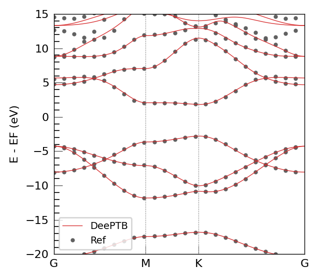
band.band_plot(emin = task_options['emin'],
emax = task_options['emax'],
ref_band = task_options['ref_band'],)
DPNEGF ERROR   TBPLaS is not installed. Thus the TBPLaS is not available, Please install it first.
/opt/mamba/envs/dpnegf-dev/lib/python3.10/site-packages/torch/nested/__init__.py:107: UserWarning: The PyTorch API of nested tensors is in prototype stage and will change in the near future. (Triggered internally at ../aten/src/ATen/NestedTensorImpl.cpp:178.)
  return torch._nested_tensor_from_tensor_list(ts, dtype, None, device, None)
DPNEGF WARNING eig_solver is not set, using default 'torch'.
DPNEGF INFO    KPOINTS  klist: 300 kpoints
DPNEGF INFO    The eigenvalues are already in data. will use them.
DPNEGF INFO    Calculating Fermi energy in the case of spin-degeneracy.
DPNEGF WARNING Fermi level bisection did not converge under tolerance 1e-10 after 57 iterations.
DPNEGF INFO    q_cal: 7.9999999708937874, total_electrons: 8.0, diff q: 2.910621255125534e-08
DPNEGF INFO    Estimated E_fermi: -3.5829840898513794 based on the valence electrons setting nel_atom : {'C': 4} .
DPNEGF INFO    No Fermi energy provided, using estimated value: -3.5830 eV
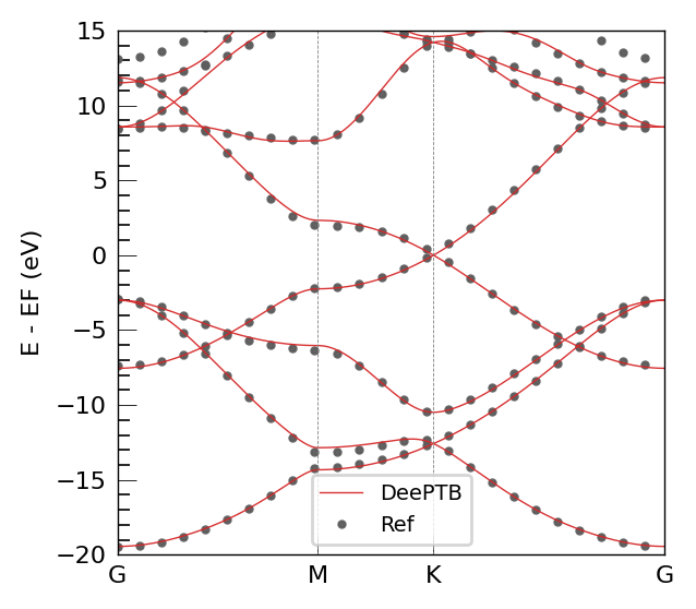
The DFT band structure demonstrates excellent agreement with the DeePTB model. Critically, the model accurately reproduces the hallmark electronic features of graphene. The Fermi level is correctly positioned at the Dirac point, located at the K high-symmetry point of the Brillouin zone. The linear dispersion near this point, forming the characteristic Dirac cone, is clearly visible and matches the reference data precisely.
1.2 Principal layers in leads#
Now we can pay attention to quantum transport simulaitons.
try:
    from dpnegf.runner.NEGF import NEGF
except ImportError as e:
    raise ImportError("dpnegf not found. Please install firstly.") from e

import json
negf_input_file =  "negf.json"
structure =  "stru_negf.xyz"

with open(negf_input_file, "r") as f:
    negf_json = json.load(f)
DPNEGF INFO Numba is available and JIT functions are compiled.
A critical component is AtomicData_options, which specifies the cutoff parameters for the model:
r_max: the cutoff value for bond considering in TB modeler_max: the cutoff value for environment correction, should set for nnsk+env correction modeloer_max: the cutoff value for onsite correction in nnsk model, need to set in strain mode
In other words, AtomicData_options determines the locality of the model, i.e., how far atomic interactions are considered in the calculation.
The code would determine the AtomicData_options automatically with DeePTB v2.2. At the same time, it can be visiualized conviently
by NEGF.update_atomicdata_options.
AtomicData_options = NEGF.update_atomicdata_options(model)
DPNEGF INFO    The AtomicData_options is:
               {
                   "r_max": {
                       "C-C": 4.99
                   },
                   "er_max": null,
                   "oer_max": 6.3
               }
The largest cutoff value determines the maximum interaction distance, which is critical for defining the lead geometry in NEGF simulations.
In DPNEGF, a key requirement of the self-energy algorithm is to define two principal layers (PLs) for each lead. Each PL must be longer than the maximum interaction distance to ensure proper treatment of interactions. That is, the PLs only include nearest-neighbor interactions.
Additionally, the algorithm requires that:
The PLs within the same lead be identical, differing only by a translation along the transport direction.
In the input structure file, the atomic coordinates of the left lead should be ordered with the 1st PL first, followed by the 2nd PL. See
/examples/graphene/stru_negf.xyzfor reference.
The following figure illustrates the device/lead region and principal layers in the lead:
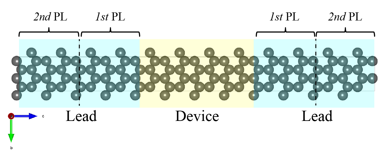
In this case, the length of PL should be larger than 6.3 Angstrom. However, too long PL is unnecessary for the computing cost. Considering both the translation requirement and nearest-neighbor interaction, we set the length of PL as 8.67 Angstrom.
Now we can strat the NEGF calculation!
1.3 NEGF calculation for graphene#
For NEGF calculation on systems with leads having periodicity along the transverse direction, it’s natural to calculate the \(k\)-resolved transmission \(T(k,E)\) and sum up for the total transmission \(T(E) = \sum_k w_k T(k,E)\) where \(w_k\) is the weight for the specified \(k\).
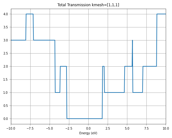
Firstly, we only consider the Gamma point calculation for graphene.
# Gamma point calculation
negf_json['task_options']["stru_options"]['kmesh'] = [1,1,1]
# Energy step and range for transmission calculation
print(f"Energy range: {negf_json['task_options']['emin']} to {negf_json['task_options']['emax']} eV, step: {negf_json['task_options']['espacing']} eV")
Energy range: -10 to 10 eV, step: 0.05 eV
Here kmesh specify the \(k\)-point mesh for transmission calculaiton.
k_mesh_lead_Ef is the \(k\)-point mesh for lead Fermi level determination.
For leads with long PLs, a sparse kmesh_lead_Ef is enough.
# Structural information for device and electrodes
negf_json['task_options']["stru_options"]
{'gamma_center': False,
 'time_reversal_symmetry': True,
 'nel_atom': {'C': 4},
 'kmesh': [1, 1, 1],
 'pbc': [False, True, False],
 'device': {'id': '32-64', 'sort': True},
 'lead_L': {'id': '0-32',
  'voltage': 0.0,
  'kmesh_lead_Ef': [1, 50, 20],
  'useBloch': False},
 'lead_R': {'id': '64-96',
  'voltage': 0.0,
  'kmesh_lead_Ef': [1, 50, 20],
  'useBloch': False}}
Now we can run the NEGF calculation ( ~2 mins in a 8-core CPU ):
output = "./negf_output"
if os.path.isdir(output):
    shutil.rmtree(output, ignore_errors=True)
os.makedirs(output, exist_ok=True)

negf = NEGF(
    model=model,
    structure=structure,
    results_path=output,
    use_saved_se=False, # whether to use the saved self-energy
    se_info_display=False,
    **negf_json['task_options']
)

negf.compute()
DPNEGF INFO ------ k-point for NEGF -----
DPNEGF INFO Gamma Center: False
DPNEGF INFO Time Reversal: True
DPNEGF INFO k-points Num: 1
DPNEGF INFO k-points: [[-0. -0. -0.]]
DPNEGF INFO k-points weights: [1.]
DPNEGF INFO --------------------------------
DPNEGF INFO The AtomicData_options is:
{
"r_max": {
"C-C": 4.99
},
"er_max": null,
"oer_max": 6.3
}
DPNEGF INFO The structure is sorted lexicographically in this version!
DPNEGF INFO Lead principal layers translational equivalence error (on average): 1.732051e-10 (threshold: 1.000000e-05)
DPNEGF INFO Lead principal layers translational equivalence error (on average): 1.732061e-10 (threshold: 1.000000e-05)
DPNEGF INFO The coupling width of lead_L is 72.
DPNEGF WARNING WARNING, the lead's hamiltonian attained from diffferent methods have slight differences RMSE = 0.0000006.
DPNEGF INFO The coupling width of lead_R is 72.
DPNEGF WARNING WARNING, the lead's hamiltonian attained from diffferent methods have slight differences RMSE = 0.0000019.
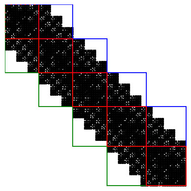
DPNEGF INFO The Hamiltonian is block tridiagonalized into 3 subblocks.
DPNEGF INFO the number of elements in subblocks: 61128
DPNEGF INFO occupation of subblocks: 73.69791666666666 %
DPNEGF INFO --------------------------------------------------------------------------------
DPNEGF INFO The Hamiltonian has been initialized by model.
DPNEGF INFO ================================================================================
DPNEGF INFO -------------Fermi level calculation-------------
DPNEGF WARNING No doping detected in lead_L, fixed_charge = 0
DPNEGF WARNING No doping detected in lead_R, fixed_charge = 0
DPNEGF INFO Number of electrons in lead_L: {'C': 4}
DPNEGF INFO Number of electrons in lead_R: {'C': 4}
DPNEGF INFO -----Calculating Fermi level for lead_L-----
DPNEGF INFO KPOINTS kmesh sampling: 535 kpoints
DPNEGF INFO Getting eigenvalues from the model.
DPNEGF INFO Calculating Fermi energy in the case of spin-degeneracy.
DPNEGF WARNING Fermi level bisection did not converge under tolerance 1e-10 after 57 iterations.
DPNEGF INFO q_cal: 128.0000000009015, total_electrons: 128.0, diff q: 9.015082014229847e-10
DPNEGF INFO Estimated E_fermi: -3.5829886198043823 based on the valence electrons setting nel_atom : {'C': 4} .
DPNEGF INFO -----Calculating Fermi level for lead_R-----
DPNEGF INFO KPOINTS kmesh sampling: 535 kpoints
DPNEGF INFO Getting eigenvalues from the model.
DPNEGF INFO Calculating Fermi energy in the case of spin-degeneracy.
DPNEGF WARNING Fermi level bisection did not converge under tolerance 1e-10 after 57 iterations.
DPNEGF INFO q_cal: 128.00000000090498, total_electrons: 128.0, diff q: 9.04975649973494e-10
DPNEGF INFO Estimated E_fermi: -3.582987666130066 based on the valence electrons setting nel_atom : {'C': 4} .
DPNEGF INFO -------------------------------------------------
DPNEGF INFO Zero bias case detected.
DPNEGF INFO Fermi level for lead_L: -3.5829886198043823
DPNEGF INFO Fermi level for lead_R: -3.582987666130066
DPNEGF INFO Electrochemical potential for lead_L: -3.5829886198043823
DPNEGF INFO Electrochemical potential for lead_R: -3.582987666130066
DPNEGF INFO Reference energy E_ref: -3.5829886198043823
DPNEGF INFO =================================================
DPNEGF INFO ------Self-energy calculation------
DPNEGF INFO Calculating self-energy and saving to ./negf_output/self_energy
DPNEGF INFO Merging 400 tmp self energy files into ./negf_output/self_energy/self_energy_leadL.h5
DPNEGF INFO Merge complete.
DPNEGF INFO Merging 400 tmp self energy files into ./negf_output/self_energy/self_energy_leadR.h5
DPNEGF INFO Merge complete.
DPNEGF INFO -----------------------------------
DPNEGF INFO Properties computation at k = [-0.0000,-0.0000,-0.0000]
DPNEGF INFO computing green's function at e = -10.000
DPNEGF INFO computing green's function at e = -7.995
DPNEGF INFO computing green's function at e = -5.990
DPNEGF INFO computing green's function at e = -3.985
DPNEGF INFO computing green's function at e = -1.980
DPNEGF INFO computing green's function at e = 0.025
DPNEGF INFO computing green's function at e = 2.030
DPNEGF INFO computing green's function at e = 4.035
DPNEGF INFO computing green's function at e = 6.040
DPNEGF INFO computing green's function at e = 8.045
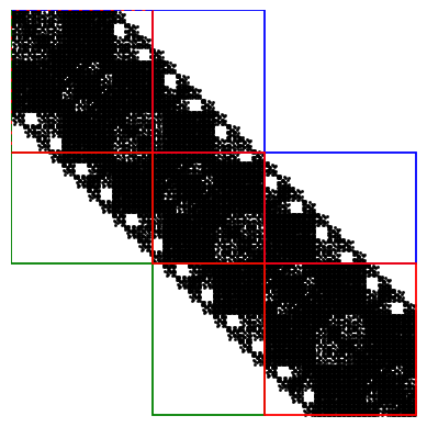
If block_tridiagonal is set to true in the input file, the block-tridiagonal Hamiltonian is used in the recursive Green’s function algorithm, as shown in this figure. This significantly accelerates the NEGF calculation, and we strongly recommend enabling this option whenever possible.
Here we can read the results through the dict negf_out:
import torch
import matplotlib.pyplot as plt
results_path = os.path.join(output, 'negf.out.pth')
if os.path.exists(results_path) is False:
    raise FileNotFoundError(f"Results file {results_path} not found. Please check if the NEGF calculation was successful.")
negf_out = torch.load(results_path,weights_only=False)
negf_out.keys()
dict_keys(['k', 'wk', 'uni_grid', 'DOS', 'T_k', 'LDOS', 'T_avg'])
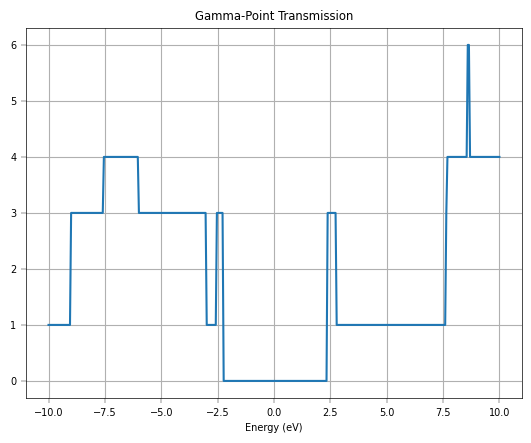
plt.plot(negf_out['uni_grid'], negf_out['T_avg'])
plt.xlabel('Energy (eV)')
plt.title('Gamma-Point Transmission')
plt.grid()
plt.show()
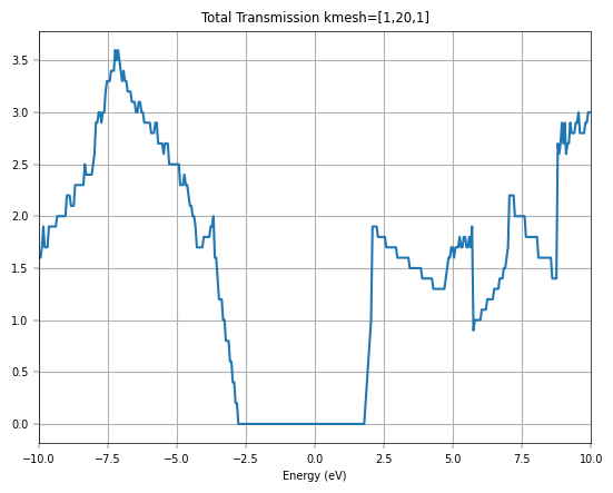
Furthermore, we increase the \(k\)-point mesh for transmission.
# Increase k-point sampling for better accuracy
negf_json['task_options']["stru_options"]['kmesh'] = [1,20,1]
For \(k\)-point mesh [1,20,1], the computation from scratch takes ~23 mins in a 8-core CPU. However, if directly loading the saved self-energies, it takes ~6 mins.
We have prepared the self-energies in negf_out_k20/self_energy and you can just run the cell with use_saved_se=True.
output = "./negf_output_k20"

negf = NEGF(
    model=model,
    structure=structure,
    results_path=output,
    use_saved_se=True,   # use the saved self-energy to speed up calculation
    **negf_json['task_options']
)

negf.compute()
output = "./negf_output_k20"
results_path = os.path.join(output, 'negf.out.pth')
if os.path.exists(results_path) is False:
raise FileNotFoundError(f"Results file {results_path} not found. Please check if the NEGF calculation was successful.")
negf_out = torch.load(results_path,weights_only=False)
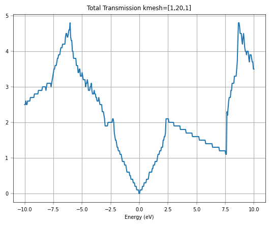
plt.plot(negf_out['uni_grid'], negf_out['T_avg'])
plt.xlabel('Energy (eV)')
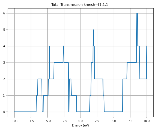
plt.title('Total Transmission kmesh=[1,20,1]')
plt.xlim(-10,10)
plt.grid()
plt.show()
If we further increase the \(k\)-point mesh density, we can get a smoother transmission curve for graphene. Considering the time, we directly plot the total transmission corresponding to \(k\)-point mesh [1,100,1], and compare it with DFT-NEGF (TranSIESTA + TBtrans).
import numpy as np
import matplotlib.pyplot as plt
import torch
output = 'negf_output_k100'
results_path = os.path.join(output, 'negf.out.pth')
if os.path.exists(results_path) is False:
    raise FileNotFoundError(f"Results file {results_path} not found. Please check if the NEGF calculation was successful.")
negf_out = torch.load(results_path,weights_only=False)
Erange_dpnegf = np.linspace(-15,15,int((15-(-15))/0.05))
tbt_trans_E = np.load(os.path.join(output, 'trans_tbt_E.npy'))
tbt_trans = np.load(os.path.join(output, 'trans_tbt_Tavg.npy'))
Ef_TS = -24.878582000732422
plt.plot(Erange_dpnegf, negf_out['T_avg'], label='DeePTB-NEGF')
plt.plot(tbt_trans_E - Ef_TS, tbt_trans,'--', label=r'DFT-NEGF')
plt.xlabel('Energy (eV)')
plt.title('Total Transmission')
plt.grid()
plt.legend(loc='upper center')
plt.xlim(-10,10)
plt.show()
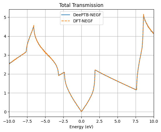
The transmission spectra further validate the model’s accuracy for transport simulations. The initial Gamma-point calculation shows integer plateaus in the transmission, which is characteristic of ballistic transport in one-dimensional channels. However, to capture the full picture of 2D transport, a summation over the transverse k-points is necessary. The final plot, which compares the total transmission from DeePTB-NEGF with that from a full DFT-NEGF calculation, shows remarkable consistency. Both methods produce the distinctive V-shaped transmission spectrum around the Fermi level, a direct consequence of graphene’s linear density of states.
2. Quantum Transport in hBN#
Here we extend DPNEGF’s application to hBN illustrating its capability to various materials.
For simpilicy, we have prepared a model in example/hBN/train/. Users can just run the same commands above to repeat the procedures.
import os
from pathlib import Path
from dptb.nn.build import build_model
from ase.io import read
from dpnegf.utils.loggers import set_log_handles
import logging
from pathlib import Path


workdir='../../examples/hBN'
wd = Path(workdir)
if not wd.is_dir():
    raise FileNotFoundError(f"Workdir '{wd}' not found. Please adjust 'workdir'.")
os.chdir(wd)
print("\t".join(sorted(os.listdir("."))))

results_path = 'band_plot_api'
log_path = os.path.join(results_path, 'log')
log_level = logging.INFO
set_log_handles(log_level, Path(log_path) if log_path else None)


model =  "./train/train_out/checkpoint/nnsk.best.pth" # the model for demonstration
model = build_model(model)

# read the structure
structure =  "./train/data/POSCAR"
atoms = read(structure)
print(atoms)
DPNEGF INFO    ================================================================================
DPNEGF INFO                                      Version Info
DPNEGF INFO    --------------------------------------------------------------------------------
DPNEGF INFO    DPNEGF               : 0.1.1.dev148+0e0863a
DPNEGF INFO    DeePTB               : 2.2.1.dev17+024a5fe
DPNEGF INFO    ================================================================================

DPNEGF INFO    The ['overlap_param'] are frozen!
DPNEGF INFO    The ['overlap_param'] are frozen!
band.json	band_plot_api	extra_baseline	negf.json	negf_output_k20	negf_output_k70	siesta.TBT.AVTRANS_Left-Right	siesta.TBT.nc	stru_negf.xyz	train
Atoms(symbols='NB', pbc=True, cell=[[2.5039999485, 0.0, 0.0], [-1.2519999743, 2.1685275665, 0.0], [0.0, 0.0, 30.0]])
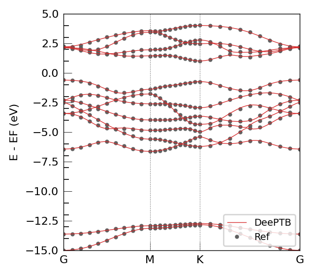
The band predicted by the model is shown:
from dptb.postprocess.bandstructure.band import Band


task_options = {
        "task": "band",
        "kline_type":"abacus",
        "kpath":[
                [0, 0, 0, 110],
                [0.5, 0, 0, 62],
                [0.3333333, 0.3333333, 0, 127],
                [0, 0, 0, 1]
                ],
        "klabels":["G", "M", "K", "G"],
        "emin":-20,
        "emax": 15,
        "nel_atom":{"B": 3,
                    "N": 5},
        "ref_band": "./train/data/kpath.0/eigenvalues.npy"

       }


band = Band(model, results_path)
AtomicData_options = { "pbc": True}
band.get_bands(data = atoms,
               kpath_kwargs = task_options,
               AtomicData_options = AtomicData_options)
band.band_plot(emin = task_options['emin'],
               emax = task_options['emax'],
               ref_band = task_options['ref_band'],)
DPNEGF ERROR   TBPLaS is not installed. Thus the TBPLaS is not available, Please install it first.
/opt/mamba/envs/dpnegf-dev/lib/python3.10/site-packages/torch/nested/__init__.py:107: UserWarning: The PyTorch API of nested tensors is in prototype stage and will change in the near future. (Triggered internally at ../aten/src/ATen/NestedTensorImpl.cpp:178.)
  return torch._nested_tensor_from_tensor_list(ts, dtype, None, device, None)
DPNEGF WARNING eig_solver is not set, using default 'torch'.
DPNEGF INFO    KPOINTS  klist: 300 kpoints
DPNEGF INFO    The eigenvalues are already in data. will use them.
DPNEGF INFO    Calculating Fermi energy in the case of spin-degeneracy.
DPNEGF INFO    Fermi energy converged after 3 iterations.
DPNEGF INFO    q_cal: 7.999999999999999, total_electrons: 8.0, diff q: 8.881784197001252e-16
DPNEGF INFO    Estimated E_fermi: -2.8933583906146634 based on the valence electrons setting nel_atom : {'B': 3, 'N': 5} .
DPNEGF INFO    No Fermi energy provided, using estimated value: -2.8934 eV
The NEGF calculation on hBN can be done:
try:
    from dpnegf.runner.NEGF import NEGF
except ImportError as e:
    raise ImportError("dpnegf not found. Please install firstly.") from e

import json
negf_input_file =  "negf.json"
structure =  "stru_negf.xyz"

with open(negf_input_file, "r") as f:
    negf_json = json.load(f)
DPNEGF INFO Numba is available and JIT functions are compiled.
AtomicData_options = NEGF.update_atomicdata_options(model)
DPNEGF INFO    The AtomicData_options is:
               {
                   "r_max": {
                       "B-B": 4.82,
                       "B-N": 4.640000000000001,
                       "N-B": 4.640000000000001,
                       "N-N": 4.45
                   },
                   "er_max": null,
                   "oer_max": 6.3
               }
import shutil
output = "./negf_output"
if os.path.isdir(output):
    shutil.rmtree(output, ignore_errors=True)
os.makedirs(output, exist_ok=True)

negf = NEGF(
    model=model,
    structure=structure,
    results_path=output,
    use_saved_se=False, # whether to use the saved self-energy
    se_info_display=False,
    **negf_json['task_options']
)

negf.compute()
DPNEGF INFO    ------ k-point for NEGF -----
DPNEGF INFO    Gamma Center: False
DPNEGF INFO    Time Reversal: True
DPNEGF INFO    k-points Num: 1
DPNEGF INFO    k-points: [[-0. -0. -0.]]
DPNEGF INFO    k-points weights: [1.]
DPNEGF INFO    --------------------------------
DPNEGF INFO    The AtomicData_options is:
               {
                   "r_max": {
                       "B-B": 4.82,
                       "B-N": 4.640000000000001,
                       "N-B": 4.640000000000001,
                       "N-N": 4.45
                   },
                   "er_max": null,
                   "oer_max": 6.3
               }
DPNEGF INFO    The structure is sorted lexicographically in this version!
DPNEGF INFO    Lead principal layers translational equivalence error (on average): 3.803219e-09 (threshold: 1.000000e-05)
DPNEGF INFO    Lead principal layers translational equivalence error (on average): 2.120221e-09 (threshold: 1.000000e-05)
DPNEGF INFO    The coupling width of lead_L is 54.
DPNEGF WARNING WARNING, the lead's hamiltonian attained from diffferent methods have slight differences   RMSE = 0.0000001.
DPNEGF INFO    The coupling width of lead_R is 54.
DPNEGF WARNING WARNING, the lead's hamiltonian attained from diffferent methods have slight differences   RMSE = 0.0000003.
DPNEGF INFO    The Hamiltonian is block tridiagonalized into 5 subblocks.
DPNEGF INFO       the number of elements in subblocks: 43092
DPNEGF INFO                   occupation of subblocks: 51.953125 %
DPNEGF INFO    --------------------------------------------------------------------------------
DPNEGF INFO    The Hamiltonian has been initialized by model.
DPNEGF INFO    ================================================================================
DPNEGF INFO    -------------Fermi level calculation-------------
DPNEGF WARNING No doping detected in lead_L, fixed_charge = 0
DPNEGF WARNING No doping detected in lead_R, fixed_charge = 0
DPNEGF INFO    Number of electrons in lead_L: {'B': 3, 'N': 5}
DPNEGF INFO    Number of electrons in lead_R: {'B': 3, 'N': 5}
DPNEGF INFO    -----Calculating Fermi level for lead_L-----
DPNEGF INFO    KPOINTS  kmesh sampling: 535 kpoints
DPNEGF INFO    Getting eigenvalues from the model.
DPNEGF INFO    Calculating Fermi energy in the case of spin-degeneracy.
DPNEGF INFO    Fermi energy converged after 3 iterations.
DPNEGF INFO    q_cal: 128.00000000000006, total_electrons: 128.0, diff q: 5.684341886080802e-14
DPNEGF INFO    Estimated E_fermi: -2.870708359971734 based on the valence electrons setting nel_atom : {'B': 3, 'N': 5} .
DPNEGF INFO    -----Calculating Fermi level for lead_R-----
DPNEGF INFO    KPOINTS  kmesh sampling: 535 kpoints
DPNEGF INFO    Getting eigenvalues from the model.
DPNEGF INFO    Calculating Fermi energy in the case of spin-degeneracy.
DPNEGF INFO    Fermi energy converged after 3 iterations.
DPNEGF INFO    q_cal: 128.00000000000006, total_electrons: 128.0, diff q: 5.684341886080802e-14
DPNEGF INFO    Estimated E_fermi: -2.870710982576104 based on the valence electrons setting nel_atom : {'B': 3, 'N': 5} .
DPNEGF INFO    -------------------------------------------------
DPNEGF INFO    Zero bias case detected.
DPNEGF INFO    Fermi level for lead_L: -2.870708359971734
DPNEGF INFO    Fermi level for lead_R: -2.870710982576104
DPNEGF INFO    Electrochemical potential for lead_L: -2.870708359971734
DPNEGF INFO    Electrochemical potential for lead_R: -2.870710982576104
DPNEGF INFO    Reference energy E_ref: -2.870708359971734
DPNEGF INFO    =================================================

DPNEGF INFO    ------Self-energy calculation------
DPNEGF INFO    Calculating self-energy and saving to ./negf_output/self_energy
DPNEGF INFO    Merging 400 tmp self energy files into ./negf_output/self_energy/self_energy_leadL.h5
DPNEGF INFO    Merge complete.
DPNEGF INFO    Merging 400 tmp self energy files into ./negf_output/self_energy/self_energy_leadR.h5
DPNEGF INFO    Merge complete.
DPNEGF INFO    -----------------------------------

DPNEGF INFO    Properties computation at k = [-0.0000,-0.0000,-0.0000]
DPNEGF INFO    computing green's function at e = -10.000
DPNEGF INFO    computing green's function at e = -7.995
DPNEGF INFO    computing green's function at e = -5.990
DPNEGF INFO    computing green's function at e = -3.985
DPNEGF INFO    computing green's function at e = -1.980
DPNEGF INFO    computing green's function at e = 0.025
DPNEGF INFO    computing green's function at e = 2.030
DPNEGF INFO    computing green's function at e = 4.035
DPNEGF INFO    computing green's function at e = 6.040
DPNEGF INFO    computing green's function at e = 8.045
import torch
import matplotlib.pyplot as plt

output = "./negf_output"
results_path = os.path.join(output, 'negf.out.pth')
if os.path.exists(results_path) is False:
    raise FileNotFoundError(f"Results file {results_path} not found. Please check if the NEGF calculation was successful.")
negf_out = torch.load(results_path,weights_only=False)

plt.plot(negf_out['uni_grid'], negf_out['T_avg'])
plt.xlabel('Energy (eV)')
plt.title('Total Transmission kmesh=[1,1,1]')
plt.xlim(-10,10)
plt.grid()
plt.show()
# Increase k-point sampling for better accuracy
negf_json['task_options']["stru_options"]['kmesh'] = [1,20,1]
It also takes about 23 minutes on an 8-core CPU.
output = "./negf_output_k20"
os.makedirs(output, exist_ok=True)

negf = NEGF(
    model=model,
    structure=structure,
    results_path=output,
    use_saved_se=False, # whether to use the saved self-energy
    se_info_display=False,
    **negf_json['task_options']
)

negf.compute()
import torch
import matplotlib.pyplot as plt

output = "./negf_output_k20"
results_path = os.path.join(output, 'negf.out.pth')
if os.path.exists(results_path) is False:
    raise FileNotFoundError(f"Results file {results_path} not found. Please check if the NEGF calculation was successful.")
negf_out = torch.load(results_path,weights_only=False)

plt.plot(negf_out['uni_grid'], negf_out['T_avg'])
plt.xlabel('Energy (eV)')
plt.title('Total Transmission kmesh=[1,20,1]')
plt.xlim(-10,10)
plt.grid()
plt.show()
# Increase k-point sampling for better accuracy
negf_json['task_options']["stru_options"]['kmesh'] = [1,70,1]
Given the computational cost, we do not recommend running this cell from scratch (it takes more than 40 minutes on a 32-core CPU). Instead, we provide precomputed self-energy files that can be loaded directly by setting use_saved_se as True. Even with this option, the process still requires about 20 minutes on a 32-core CPU.
output = "./negf_output_k70"
os.makedirs(output, exist_ok=True)

negf = NEGF(
    model=model,
    structure=structure,
    results_path=output,
    use_saved_se=True, # whether to use the saved self-energy
    se_info_display=False,
    **negf_json['task_options']
)

negf.compute()
The transmission spectra obtained from DFT-NEGF and DPNEGF show excellent agreement.
import torch
import matplotlib.pyplot as plt
import numpy as np

output = "./negf_output_k70"
results_path = os.path.join(output, 'negf.out.pth')
if os.path.exists(results_path) is False:
    raise FileNotFoundError(f"Results file {results_path} not found. Please check if the NEGF calculation was successful.")
negf_out = torch.load(results_path,weights_only=False)


data = np.loadtxt('./siesta.TBT.AVTRANS_Left-Right', comments="#")
E_tbt = data[:, 0]   # eV
T_tbt = data[:, 1]   # G0

energy_shift = 0.65 # arising from the different Fermi level algorithm; for semiconductor, the Fermi level is arbitrary in the gap.

plt.plot(negf_out['uni_grid'] , negf_out['T_avg'],label='DPNEGF')
plt.plot(E_tbt + energy_shift, T_tbt,'--', label=r'DFT-NEGF')
plt.xlabel('Energy (eV)')
plt.title('Total Transmission kmesh=[1,70,1]')
plt.xlim(-10,10)
plt.ylim(0,4)
plt.grid()
plt.legend(loc='upper center')
plt.show()
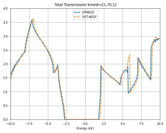
The transmission spectrum of hBN clearly shows a wide plateau of zero transmission around the Fermi level. This feature directly corresponds to the band gap observed in the previously calculated electronic band structure.
3. Quantum Transport in MoS2#
DPNEGF can perform NEGF calculations using electronic structures from any DFT software. For codes without NEGF support (e.g., plane-wave DFT such as VASP), DeePTB extracts the electronic outputs and converts them into NEGF-ready Hamiltonians. Compared with Wannierization, DeePTB offers a faster and more transferable way to construct Hamiltonians.
Here, we use the MoS2 band structure from ABACUS and compute the corresponding transmission spectrum, demonstrating how DPNEGF enables NEGF analysis even when the original DFT code does not provide it.
import os
from pathlib import Path
from dptb.nn.build import build_model
from ase.io import read
from dpnegf.utils.loggers import set_log_handles
import logging
from pathlib import Path


workdir='../../examples/MoS2'
wd = Path(workdir)
if not wd.is_dir():
    raise FileNotFoundError(f"Workdir '{wd}' not found. Please adjust 'workdir'.")
os.chdir(wd)
print("\t".join(sorted(os.listdir("."))))

results_path = 'band_plot_api'
log_path = os.path.join(results_path, 'log')
log_level = logging.INFO
set_log_handles(log_level, Path(log_path) if log_path else None)


model =  "./train/train_out/checkpoint/nnsk.best.pth" # the model for demonstration
model = build_model(model)

# read the structure
structure =  "./train/data/POSCAR"
atoms = read(structure)
print(atoms)
DPNEGF INFO    ================================================================================
DPNEGF INFO                                      Version Info
DPNEGF INFO    --------------------------------------------------------------------------------
DPNEGF INFO    DPNEGF               : 0.1.1.dev148+0e0863a
DPNEGF INFO    DeePTB               : 2.2.1.dev17+024a5fe
DPNEGF INFO    ================================================================================

DPNEGF INFO    The ['overlap_param'] are frozen!
DPNEGF INFO    The ['overlap_param'] are frozen!
MoS2_orth.vasp	MoS2_unit_rlx.vasp	POSCAR	band_plot_api	extra_baseline	negf.json	negf_output	orth_ckpt_r_max_5.3_sk.json	stru_negf.xyz	train
Atoms(symbols='MoS2', pbc=True, cell=[[3.1911949999999996, 0.0, 0.0], [-1.595598, 2.763656, 0.0], [-0.0, -0.0, 18.12711]], momenta=...)
from dptb.postprocess.bandstructure.band import Band


task_options = {
        "task": "band",
        "kline_type":"abacus",
        "kpath":[
            [0, 0, 0, 30],
            [0.5, 0, 0, 30],
            [0.3333333, 0.3333333, 0, 30],
            [0, 0, 0, 1]
        ],
        "klabels":["G", "M", "K", "G"],
        "emin":-15,
        "emax":5,
        "nel_atom":{"Mo":6,"S":6},
        "ref_band": "./train/data/kpath.0/eigenvalues.npy"

       }


band = Band(model, results_path)
AtomicData_options = { "pbc": True}
band.get_bands(data = atoms,
               kpath_kwargs = task_options,
               AtomicData_options = AtomicData_options)
band.band_plot(emin = task_options['emin'],
               emax = task_options['emax'],
               ref_band = task_options['ref_band'],)
DPNEGF WARNING eig_solver is not set, using default 'torch'.
DPNEGF INFO    KPOINTS  klist: 91 kpoints
DPNEGF INFO    The eigenvalues are already in data. will use them.
DPNEGF INFO    Calculating Fermi energy in the case of spin-degeneracy.
DPNEGF INFO    Fermi energy converged after 3 iterations.
DPNEGF INFO    q_cal: 18.0, total_electrons: 18.0, diff q: 0.0
DPNEGF INFO    Estimated E_fermi: -3.256112973973428 based on the valence electrons setting nel_atom : {'Mo': 6, 'S': 6} .
DPNEGF INFO    No Fermi energy provided, using estimated value: -3.2561 eV
try:
    from dpnegf.runner.NEGF import NEGF
except ImportError as e:
    raise ImportError("dpnegf not found. Please install firstly.") from e

import json
negf_input_file =  "negf.json"
structure =  "stru_negf.xyz"

with open(negf_input_file, "r") as f:
    negf_json = json.load(f)
AtomicData_options = NEGF.update_atomicdata_options(model)
DPNEGF INFO    The AtomicData_options is:
               {
                   "r_max": {
                       "S-S": 6.26,
                       "S-Mo": 6.449999999999999,
                       "Mo-S": 6.449999999999999,
                       "Mo-Mo": 6.630000000000001
                   },
                   "er_max": null,
                   "oer_max": 6.3
               }
# Increase k-point sampling for better accuracy
negf_json['task_options']["stru_options"]['kmesh'] = [1,1,1]
import shutil
output = "./negf_output"
if os.path.isdir(output):
    shutil.rmtree(output, ignore_errors=True)
os.makedirs(output, exist_ok=True)

negf = NEGF(
    model=model,
    structure=structure,
    results_path=output,
    use_saved_se=False, # whether to use the saved self-energy
    se_info_display=False,
    **negf_json['task_options']
)

negf.compute()
DPNEGF INFO    ------ k-point for NEGF -----
DPNEGF INFO    Gamma Center: False
DPNEGF INFO    Time Reversal: True
DPNEGF INFO    k-points Num: 1
DPNEGF INFO    k-points: [[-0. -0. -0.]]
DPNEGF INFO    k-points weights: [1.]
DPNEGF INFO    --------------------------------
DPNEGF INFO    The AtomicData_options is:
               {
                   "r_max": {
                       "S-S": 6.26,
                       "S-Mo": 6.449999999999999,
                       "Mo-S": 6.449999999999999,
                       "Mo-Mo": 6.630000000000001
                   },
                   "er_max": null,
                   "oer_max": 6.3
               }
DPNEGF INFO    The structure is sorted lexicographically in this version!
DPNEGF INFO    Lead principal layers translational equivalence error (on average): 2.849356e-09 (threshold: 1.000000e-05)
DPNEGF INFO    Lead principal layers translational equivalence error (on average): 4.413665e-09 (threshold: 1.000000e-05)
DPNEGF INFO    The coupling width of lead_L is 54.
DPNEGF WARNING WARNING, the lead's hamiltonian attained from diffferent methods have slight differences   RMSE = 0.0000001.
DPNEGF INFO    The coupling width of lead_R is 54.
DPNEGF INFO    The Hamiltonian is block tridiagonalized into 3 subblocks.
DPNEGF INFO       the number of elements in subblocks: 34992
DPNEGF INFO                   occupation of subblocks: 75.0 %
DPNEGF INFO    --------------------------------------------------------------------------------
DPNEGF INFO    The Hamiltonian has been initialized by model.
DPNEGF INFO    ================================================================================
DPNEGF INFO    -------------Fermi level calculation-------------
DPNEGF WARNING No doping detected in lead_L, fixed_charge = 0
DPNEGF WARNING No doping detected in lead_R, fixed_charge = 0
DPNEGF INFO    Number of electrons in lead_L: {'Mo': 6, 'S': 6}
DPNEGF INFO    Number of electrons in lead_R: {'Mo': 6, 'S': 6}
DPNEGF INFO    -----Calculating Fermi level for lead_L-----
DPNEGF INFO    KPOINTS  kmesh sampling: 535 kpoints
DPNEGF INFO    Getting eigenvalues from the model.
DPNEGF INFO    Calculating Fermi energy in the case of spin-degeneracy.
DPNEGF INFO    Fermi energy converged after 3 iterations.
DPNEGF INFO    q_cal: 144.00000000000003, total_electrons: 144.0, diff q: 2.842170943040401e-14
DPNEGF INFO    Estimated E_fermi: -3.2348815338761527 based on the valence electrons setting nel_atom : {'Mo': 6, 'S': 6} .
DPNEGF INFO    -----Calculating Fermi level for lead_R-----
DPNEGF INFO    KPOINTS  kmesh sampling: 535 kpoints
DPNEGF INFO    Getting eigenvalues from the model.
DPNEGF INFO    Calculating Fermi energy in the case of spin-degeneracy.
DPNEGF INFO    Fermi energy converged after 3 iterations.
DPNEGF INFO    q_cal: 144.00000000000003, total_electrons: 144.0, diff q: 2.842170943040401e-14
DPNEGF INFO    Estimated E_fermi: -3.234879864946099 based on the valence electrons setting nel_atom : {'Mo': 6, 'S': 6} .
DPNEGF INFO    -------------------------------------------------
DPNEGF INFO    Zero bias case detected.
DPNEGF INFO    Fermi level for lead_L: -3.2348815338761527
DPNEGF INFO    Fermi level for lead_R: -3.234879864946099
DPNEGF INFO    Electrochemical potential for lead_L: -3.2348815338761527
DPNEGF INFO    Electrochemical potential for lead_R: -3.234879864946099
DPNEGF INFO    Reference energy E_ref: -3.2348815338761527
DPNEGF INFO    =================================================

DPNEGF INFO    ------Self-energy calculation------
DPNEGF INFO    Calculating self-energy and saving to ./negf_output/self_energy
DPNEGF INFO    Merging 400 tmp self energy files into ./negf_output/self_energy/self_energy_leadL.h5
DPNEGF INFO    Merge complete.
DPNEGF INFO    Merging 400 tmp self energy files into ./negf_output/self_energy/self_energy_leadR.h5
DPNEGF INFO    Merge complete.
DPNEGF INFO    -----------------------------------

DPNEGF INFO    Properties computation at k = [-0.0000,-0.0000,-0.0000]
DPNEGF INFO    computing green's function at e = -10.000
DPNEGF INFO    computing green's function at e = -7.995
DPNEGF INFO    computing green's function at e = -5.990
DPNEGF INFO    computing green's function at e = -3.985
DPNEGF INFO    computing green's function at e = -1.980
DPNEGF INFO    computing green's function at e = 0.025
DPNEGF INFO    computing green's function at e = 2.030
DPNEGF INFO    computing green's function at e = 4.035
DPNEGF INFO    computing green's function at e = 6.040
DPNEGF INFO    computing green's function at e = 8.045

import torch
import matplotlib.pyplot as plt

output = "./negf_output"
results_path = os.path.join(output, 'negf.out.pth')
if os.path.exists(results_path) is False:
    raise FileNotFoundError(f"Results file {results_path} not found. Please check if the NEGF calculation was successful.")
negf_out = torch.load(results_path,weights_only=False)

plt.plot(negf_out['uni_grid'], negf_out['T_avg'])
plt.xlabel('Energy (eV)')
plt.title('Total Transmission kmesh=[1,1,1]')
# plt.xlim(-5,5)
plt.grid()
plt.show()