Tutorial 1: Quantum Transport in a One-Dimensional Chain#
Introduction#
DPNEGF is a Python package that integrates the Deep Learning Tight-Binding (DeePTB) approach with the Non-Equilibrium Green’s Function (NEGF) method, establishing an efficient quantum transport simulation framework DeePTB-NEGF with first-principles accuracy.
Based on the accurate electronic structure prediction in large-scale and complex systems, DPNEGF implements the high-efficiency algorithm for high-throughput and large-scale quantum transport simulations in nanoelectronics.
Learning Objectives#
In this tutorial, you will learn
how to load DeePTB model and plot band structure
how to calculate the transmission spectrum
For demonstration, we use a one-dimensional chain as an example.
Requirements#
DeePTB and DPNEGF installed. Detailed installation instructions can be found in README.
WARM UP: A short introduction to NEGF#
The Non-Equilibrium Green’s Function (NEGF) method is a widely used theoretical framework
for studying quantum transport in nanoscale devices (molecular junctions, nanowires, CNT-FETs, etc.).
It provides a rigorous way to compute current, density of states (DOS), and transmission by combining
quantum mechanics with open boundary conditions.
1. Partitioning the system#
We divide the full system into three regions:
Left electrode (L): semi-infinite periodic lead
Device region (D): finite scattering region of interest
Right electrode ®: semi-infinite periodic lead
The Hamiltonian of the total system can be written schematically as:
2. Green’s function of the device#
The central object is the retarded Green’s function of the device region:
where:
\(H_D\): device Hamiltonian,
\(\Sigma_{L/R}^r(E)\): electrode retarded self-energies, describing the coupling between device and semi-infinite electrodes.
The self-energy contains information about level broadening induced by the leads.
3. Transmission function#
The transmission probability at energy (E) is given by:
with:
\(\Gamma_{L/R}(E) = i \big[ \Sigma_{L/R}^r(E) - \Sigma_{L/R}^a(E) \big]\) (level broadening matrices),
\(G^a(E) = \big(G^r(E)\big)^\dagger\).
4. Current (Landauer–Büttiker formula)#
The current under bias voltage \(V\) is obtained by integrating the transmission over energy:
where \(f_{L/R}(E)\) are Fermi–Dirac distributions of the electrodes (shifted by bias).
5. Key physical quantities#
DOS: density of states, related to the spectral function \(A(E) = i(G^r - G^a)\).
LDOS: local density of states, giving spatially resolved information inside the device.
Transmission spectrum: energy-resolved measure of electron transport capability.
NEGF connects microscopic Hamiltonians (from first principles or tight-binding) with observable transport quantities (DOS, current), incorporating the quantum effects naturally. This makes it an essential tool for nanoelectronics and quantum device simulations.
In DPNEGF, the DeePTB model (either DeePTB-SK or DeePTB-E3) is employed to predict the electronic Hamiltonian with first-principles accuracy, after which the efficiently implemented NEGF method is used to calculate quantum transport properties.
1. Model loading and band plotting#
In this section we will:
Load a pretrained DeePTB model for a linear atomic chain,
Plot the band structure (expected: a cosine-like dispersion for a single orbital 1D chain).
For demonstration, here we prepare a Slater-Koster Tight-Binding model with one single orbital at each atomic site.
Since there is a built-in baseline model covering the periodic table, for any target system of your interest, you can extract the corresponding model from this built-in baseline model. For more details about DeePTB and the built-in baseline model, please see DeePTB-Tutorial 1: DeePTB-SK Baseline Model.
Switch to the tutorial input directory. The examples and input files used in this tutorial are stored under examples/atomic_chain_api/input_files.
import os
from pathlib import Path
workdir='../../examples/atomic_chain_api/input_files'
wd = Path(workdir)
if not wd.is_dir():
    raise FileNotFoundError(f"Workdir '{wd}' not found. Please adjust 'workdir'.")
os.chdir(wd)
print("\t".join(sorted(os.listdir("."))))
chain.vasp negf_chain_new.json nnsk_C_new.json
The logging settings.
from dpnegf.utils.loggers import set_log_handles
import logging
from pathlib import Path


results_path = '../band_plot'
log_path = os.path.join(results_path, 'log')
log_level = logging.INFO
set_log_handles(log_level, Path(log_path) if log_path else None)
---------------------------------------------------------------------------
ModuleNotFoundError                       Traceback (most recent call last)
Cell In[2], line 1
----> 1 from dpnegf.utils.loggers import set_log_handles
      2 import logging
      3 from pathlib import Path

ModuleNotFoundError: No module named 'dpnegf'
Load model from file.
from dptb.nn.build import build_model
import json
model =  "nnsk_C_new.json" # the model for demonstration
with open(model) as f:
    model_json = json.load(f)
model = build_model(model,
                    model_options= model_json['model_options'],
                    common_options=model_json['common_options'])
DPNEGF WARNING The model option atomic_radius in nnsk is not defined in input model_options, set to v1.
After the model is loaded, bands for specific structures can be plotted.
Here we load the full system and split it into unit cell.
from ase.io import read
structure =  "chain.vasp"
atoms = read(structure)
atoms
Atoms(symbols='C12', pbc=True, cell=[10.0, 10.0, 19.2])
uni_cell_atoms = atoms[0:1]
uni_cell_atoms.cell[2][2] = atoms.cell[2][2]/len(atoms)
uni_cell_atoms
Atoms(symbols='C', pbc=True, cell=[10.0, 10.0, 1.5999999999999999])
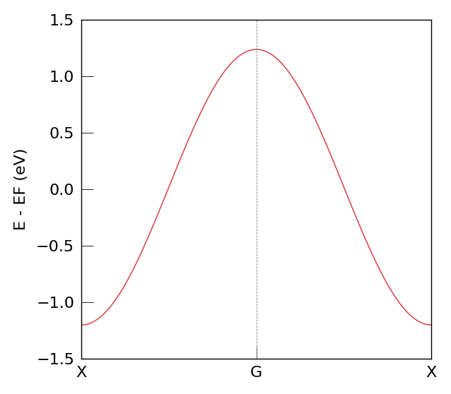
Because we only consider one orbital per atomic site, each atom contributes a single valence electron in the model.
As visible in the band diagram, the characteristic cosine-like dispersion of a one-dimensional chain appears.
from dptb.postprocess.bandstructure.band import Band
import shutil

task_options = {
        "task": "band",
        "kline_type":"abacus",
        "kpath":[[0.0,   0.0,   0.5,   50],
                 [0.0,   0.0,   0.0,   50],
                 [0.0,   0.0,  -0.5,   1]
                ],
        "klabels":["X","G","X"],
        "emin":-1.5,
        "emax": 1.5,
        "nel_atom":{"C": 1}

       }

if os.path.isdir(results_path):
    shutil.rmtree(results_path, ignore_errors=True)

band = Band(model, results_path)
AtomicData_options = {"r_max": 3.0, "pbc": True}
band.get_bands(data = uni_cell_atoms,
               kpath_kwargs = task_options,
               AtomicData_options = AtomicData_options)
band.band_plot(emin = task_options['emin'],
               emax = task_options['emax'])
DPNEGF ERROR   TBPLaS is not installed. Thus the TBPLaS is not available, Please install it first.
DPNEGF WARNING Overwrite the r_max setting in the model with the r_max setting in the AtomicData_options: 3.0
DPNEGF WARNING This is very dangerous, please make sure you know what you are doing.
/opt/mamba/envs/dpnegf-dev/lib/python3.10/site-packages/torch/nested/__init__.py:107: UserWarning: The PyTorch API of nested tensors is in prototype stage and will change in the near future. (Triggered internally at ../aten/src/ATen/NestedTensorImpl.cpp:178.)
  return torch._nested_tensor_from_tensor_list(ts, dtype, None, device, None)
DPNEGF WARNING eig_solver is not set, using default 'torch'.
DPNEGF INFO    KPOINTS  klist: 101 kpoints
DPNEGF INFO    The eigenvalues are already in data. will use them.
DPNEGF INFO    Calculating Fermi energy in the case of spin-degeneracy.
DPNEGF INFO    Fermi energy converged after 18 iterations.
DPNEGF INFO    q_cal: 0.9999982678381729, total_electrons: 1.0, diff q: 1.7321618270838002e-06
DPNEGF INFO    Estimated E_fermi: -13.65731141812973 based on the valence electrons setting nel_atom : {'C': 1} .
DPNEGF INFO    No Fermi energy provided, using estimated value: -13.6573 eV
2. NEGF calculation#
After the model is loaded, we can calculate the transmission spectrum for the one-dimension chain.
A sample input file negf_chain_new.json is provided and can be loaded directly.
try:
    from dpnegf.runner.NEGF import NEGF
except ImportError as e:
    raise ImportError("dpnegf not found. Please install firstly.") from e

negf_input_file =  "negf_chain_new.json"
structure =  "chain.vasp"
output = "../negf_output"
if os.path.isdir(output):
    shutil.rmtree(output, ignore_errors=True)
os.makedirs(output, exist_ok=True)

with open(negf_input_file, "r") as f:
    negf_json = json.load(f)
DPNEGF INFO Numba is available and JIT functions are compiled.
This input file contains:
Energy range and step for the transmission calculation,
Structural information that determines how to divide the system into device and electrode regions (left and right),
Other important parameters such as the number of valence electrons per element (the
nel_atomfield), which affects charge counting and Fermi level.
# Energy step and range for transmission calculation
negf_json['task_options']['espacing'], negf_json['task_options']['emin'], negf_json['task_options']['emax']
(0.02, -1.5, 1.5)
# Structural information for device and electrodes
negf_json['task_options']["stru_options"]
{'gamma_center': True,
 'time_reversal_symmetry': True,
 'nel_atom': {'C': 1.0},
 'kmesh': [1, 1, 1],
 'pbc': [False, False, False],
 'device': {'id': '4-8', 'sort': True},
 'lead_L': {'id': '0-4',
  'voltage': 0.0,
  'kmesh_lead_Ef': [1, 1, 20],
  'useBloch': False},
 'lead_R': {'id': '8-12',
  'voltage': 0.0,
  'kmesh_lead_Ef': [1, 1, 20],
  'useBloch': False}}
Running NEGF from API#
Note that the calculation of self-energy files may take some time.
if os.path.isdir(output):
    shutil.rmtree(output, ignore_errors=True)
os.makedirs(output)

negf = NEGF(
    model=model,
    AtomicData_options=negf_json['AtomicData_options'],
    structure=structure,
    results_path=output,
    **negf_json['task_options']
)

negf.compute()
DPNEGF INFO    ------ k-point for NEGF -----
DPNEGF INFO    Gamma Center: True
DPNEGF INFO    Time Reversal: True
DPNEGF INFO    k-points Num: 1
DPNEGF INFO    k-points: [[0 0 0]]
DPNEGF INFO    k-points weights: [1.]
DPNEGF INFO    --------------------------------
DPNEGF WARNING AtomicData_options is extracted from input file. This may be not consistent with the model options. Please be careful and check the cutoffs.
DPNEGF INFO    The AtomicData_options is:
               {
                   "r_max": 3.0
               }
DPNEGF INFO    Lead principal layers translational equivalence error (on average): 1.732052e-10 (threshold: 1.000000e-05)
DPNEGF INFO    Lead principal layers translational equivalence error (on average): 1.732051e-10 (threshold: 1.000000e-05)
DPNEGF INFO    The coupling width of lead_L is 1.
DPNEGF INFO    The coupling width of lead_R is 1.
DPNEGF INFO    --------------------------------------------------------------------------------
DPNEGF INFO    The Hamiltonian has been initialized by model.
DPNEGF INFO    ================================================================================
DPNEGF INFO    -------------Fermi level calculation-------------
DPNEGF WARNING No doping detected in lead_L, fixed_charge = 0
DPNEGF WARNING No doping detected in lead_R, fixed_charge = 0
DPNEGF INFO    Number of electrons in lead_L: {'C': 1.0}
DPNEGF INFO    Number of electrons in lead_R: {'C': 1.0}
DPNEGF INFO    -----Calculating Fermi level for lead_L-----
DPNEGF INFO    KPOINTS  kmesh sampling: 11 kpoints
DPNEGF WARNING Overwrite the r_max setting in the model with the r_max setting in the AtomicData_options: 3.0
DPNEGF WARNING This is very dangerous, please make sure you know what you are doing.
DPNEGF INFO    Getting eigenvalues from the model.
DPNEGF INFO    Calculating Fermi energy in the case of spin-degeneracy.
DPNEGF WARNING Fermi level bisection did not converge under tolerance 1e-10 after 51 iterations.
DPNEGF INFO    q_cal: 3.999994485346824, total_electrons: 4.0, diff q: 5.514653175886508e-06
DPNEGF INFO    Estimated E_fermi: -13.638588428497314 based on the valence electrons setting nel_atom : {'C': 1.0} .
DPNEGF INFO    -----Calculating Fermi level for lead_R-----
DPNEGF INFO    KPOINTS  kmesh sampling: 11 kpoints
DPNEGF WARNING Overwrite the r_max setting in the model with the r_max setting in the AtomicData_options: 3.0
DPNEGF WARNING This is very dangerous, please make sure you know what you are doing.
DPNEGF INFO    Getting eigenvalues from the model.
DPNEGF INFO    Calculating Fermi energy in the case of spin-degeneracy.
DPNEGF WARNING Fermi level bisection did not converge under tolerance 1e-10 after 51 iterations.
DPNEGF INFO    q_cal: 4.000002782981872, total_electrons: 4.0, diff q: 2.7829818716185173e-06
DPNEGF INFO    Estimated E_fermi: -13.638587474822998 based on the valence electrons setting nel_atom : {'C': 1.0} .
DPNEGF INFO    -------------------------------------------------
DPNEGF INFO    Zero bias case detected.
DPNEGF INFO    Fermi level for lead_L: -13.638588428497314
DPNEGF INFO    Fermi level for lead_R: -13.638587474822998
DPNEGF INFO    Electrochemical potential for lead_L: -13.638588428497314
DPNEGF INFO    Electrochemical potential for lead_R: -13.638587474822998
DPNEGF INFO    Reference energy E_ref: -13.638588428497314
DPNEGF INFO    =================================================

DPNEGF INFO    Merging 150 tmp self energy files into ../negf_output/self_energy/self_energy_leadL.h5
DPNEGF INFO    Merge complete.
DPNEGF INFO    Merging 150 tmp self energy files into ../negf_output/self_energy/self_energy_leadR.h5
DPNEGF INFO    Merge complete.
DPNEGF INFO    Properties computation at k = [0.0000,0.0000,0.0000]
DPNEGF INFO    computing green's function at e = -1.500
DPNEGF INFO    computing green's function at e = -1.198
DPNEGF INFO    computing green's function at e = -0.896
DPNEGF INFO    computing green's function at e = -0.594
DPNEGF INFO    computing green's function at e = -0.292
DPNEGF INFO    computing green's function at e = 0.010
DPNEGF INFO    computing green's function at e = 0.312
DPNEGF INFO    computing green's function at e = 0.614
DPNEGF INFO    computing green's function at e = 0.916
DPNEGF INFO    computing green's function at e = 1.218
Running NEGF from the Command Line#
The NEGF calculation can also be executed via the command-line interface (CLI). This allows batch runs and straightforward integration with job scripts on HPC systems.
See the example CLI commands below.
# Command line for DPNEGF
! pwd
! [ -d "../negf_output_cli" ] && rm -r ../negf_output_cli
! dpnegf run negf_chain_new.json  -i nnsk_C_new.json -stu chain.vasp -o ../negf_output_cli
Results Analysis#
We can inspect the outputs of the NEGF run by loading the results file (negf.out.pth). The output contains:
T_avg: the total transmission as a function of energy,T_k: k-point resolved transmission (if k-sampling is used),DOS: density of states on the energy grid,LDOS: local density of states defined for each atomic site.
import torch
import matplotlib.pyplot as plt
results_path = os.path.join(output, 'negf.out.pth')
if os.path.exists(results_path) is False:
    raise FileNotFoundError(f"Results file {results_path} not found. Please check if the NEGF calculation was successful.")
negf_out = torch.load(results_path,weights_only=False)
The result file is a dict containing all the results.
negf_out.keys()
dict_keys(['k', 'wk', 'uni_grid', 'DOS', 'T_k', 'LDOS', 'T_avg'])
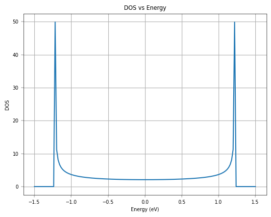
plt.plot(negf_out['uni_grid'], negf_out['DOS'][str(negf_out['k'][0])])
plt.xlabel('Energy (eV)')
plt.ylabel('DOS')
plt.title('DOS vs Energy')
plt.grid()
plt.show()
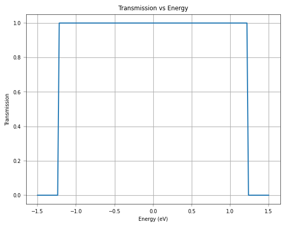
plt.plot(negf_out['uni_grid'], negf_out['T_avg'])
plt.xlabel('Energy (eV)')
plt.ylabel('Transmission')
plt.title('Transmission vs Energy')
plt.grid()
plt.show()